
Regression Lines
Chapter 2 - Day 7 - Lesson 2.5
Chapter 2
Day 1
Day 2
Day 3
Day 4
Day 5
Day 6
Day 7
Day 8
Day 9
Day 10
Day 11
Day 12
Day 13
Day 14
All Chapters
Learning Targets
-
Make predictions using regression lines, keeping in mind the dangers of extrapolation.
-
Calculate and interpret a residual.
-
Interpret the slope and y intercept of a regression line.
Activity: How Good Are Predictions Using The Barbie Data?
Activity:


Answer Key:
This activity connected back to the opening activity for Chapter 2. We started by telling the students that we had a hole in our data because someone in the group forgot to record the value for 5 rubber bands….so we are just going to make our best prediction. We started by just having students look at the numbers.
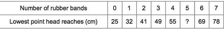
Of course students realized that our prediction should be between 55 and 69 cm. But then some students started to realize that each time a rubber ban was added, the lowest point seem to increase about 7 or 8 cm each time, so they wanted to add 8 to 55. Others wanted to find the midpoint between 55 and 69. This is all good thinking about linear relationships and slope.
Students than used the Applet to find the least squares regression line (they don’t know what “least squares” means until tomorrow). Then they compared their prediction to the actual value (somehow we found the lost data). Students are calculating a residual here without knowing this new vocabulary. We introduced the vocabulary at the end of the activity when we were summarizing.
The rest of the activity deals with the slope and y-intercept of the least squares regression line. This is a great algebra review for students.


The Barbie data is a great context for slope and y-intercept because they both have a very tangible physical meaning. The slope of the regression line tells us that for every additional rubber band added, we predict the distance that Barbie’s head reaches to increase by 7.646 cm. They y-intercept tells us the predicted lowest point that Barbie’s head reaches is 25.333 cm when there are 0 rubber bands. Of course this is really just a predicted value of Barbie’s height.
Notes
When we have students write out the equation for the least squares regression line, we have them (1) use context instead of x and y and (2) put a “hat” over the y variable to indicate that we are predicting y from x.
predicted lowest height=25.333+7.464(# rubber bands)
These two small changes will make predictions and residuals come much easier for students.
To help students remember the correct interpretation of slope, we took them back to Algebra 1, where they learned slope as rise/run or (change in y)/(change in x). Then we took our slope of 7.464 and wrote it as 7.464/1. When students think of slope as (change in y)/(change in x), the interpretation becomes much easier to come up with (rather than memorize!). We also made sure that students were saying “predicted lowest point” rather than just “lowest point” when interpreting slope and y-intercept.
You can preview tomorrow’s lesson by asking students how they think the Applet is figuring out which line is the “best”. You can also preview Lesson 2.7 by making students aware of the s (standard deviation of the residuals) and r2 (coefficient of determination), both of which will be interpreted later.